Inference and planning on factor graphs
This document is available as
- pdf http://www.marc-toussaint.net/06-infer/index.pdf
- html http://www.marc-toussaint.net/06-infer/index.html
Software is available via subversion from
- http://sourceforge.net/projects/infer
- svn co https://infer.svn.sourceforge.net/svnroot/infer infer
Contents
- Mission
- Related pages
- Inference and belief propagation in a nutshell
- The factor graph data structure and generic operations
- The data structure - a factor graph
- States of the data structure
- Message exchange
- Approximate message exchange
- Approximate message exchange (e.g., expectation propagation / assume density filtering)
- Mean field approximations
- Particle filtering
- Factors
- Generic operations and testing
- Factor types
- Tables
- Gaussians
- Mixture of Gaussians
- Unscented Transform Gaussian factor
- Linearized Function Gaussian factor
- Switch factors for relational/logic models
- Decision tree factor
- Particle factors
- Appendix: Gaussians
Mission
I am interested in a new approach to planning and motor control based on probabilistic inference techniques. This approaches aims at solving planning and control problems on structured domains - structured means that multiple state variables exist and that the system dynamics is described by some Dynamic Bayesian Network (which can express factorial, hierarchical, and mixed discrete/continuous domains). Inference techniques such as belief propagation, variational techniques or particle based approach can then be used to solve control and planning problems (solve MDPs/POMDPs).
The goals of this document are to
- provide a reference for factor graphs, message passing, and
specific factor instantiations that can directly be translated to
the implementation in the library,
- collect resources and pointers to existing inference software and related pages.
Current state
- basic low level computations with Gaussians etc are robust
- simple DBNs (HMMs, Kalman filters, switching state space models with MoGs) tested and work
- generic unit testing for factor implementations: Tables, Gaussians pass fully, MoGs and locally-linear-Gaussians pass approximately.
Software profile
The software will implement inference on factor graphs in a quite generic way, based on a virtual definition of factors. At least the following algorithms should thereby becomes special cases:
- message passing algorithms such as Belief Propagation (BP),
Loopy BP, Junction Tree, BP with any order of message exchanges
- Expectation Propagation, Gaussian (Kalman) filters/smoothers,
all message exchange schemes as above with Gaussian variables,
mixture-of-Gaussians, and factors that implement
`quasi-non-linear' dependencies between Gaussian variables (using
local-linearization or the Unscented Transform)
- Variational approximation, extraction of submodels (e.g., a
single variable Markov chain from a DBN), Factorial Hidden Markov
Models
- Particle representations - not yet
Concerning the style of implementation, the software is meant for scientists that are familiar with the theoretical background. Special aims are
- to provide a basic data structure for describing probabilistic
models that is clear, transparent, and as general as possible
- algorithms that realize inference algorithms in a generic way -
trying to be rather independent of the type of variables and
factors/conditional probabilities in the model (independent of
whether they are tables, Gaussians, MoGs, etc)
- algorithms that manipulate models, i.e., take the factor graph as an input and return a new one, e.g. to implement extraction of sub-models
Related pages
A great overview over existing inference software is given by
- Kevin Murphy
A selection of software is the following:
- Bayes Net Toolbox (BNT)
- - Kevin Murphy
A Matlab toolbox.
- Graphical Model Tool Kit (GMTK)
- - Jeff Blimes
http://ssli.ee.washington.edu/~bilmes/gmtk/
- Probabilistic Network Library (PNL)
- - Intel
http://www.intel.com/technology/computing/pnl/index.htm
C++ version of the BNT. Kevin Murphy is involved.
- Tayla Meltzer's c-inference
-
http://www.cs.huji.ac.il/~talyam/inference.html
This inspired me most: Simple and very clean implementation of various algorithms based on factor graphs (mainly used to represent Markov Random Fields
- Rebel
http://choosh.ece.ogi.edu/rebel/
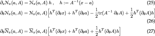
Inference and belief propagation in a nutshell
- This is a far too brief and maybe obscure intro to BP. Its origin was me trying to explain BP in a single lecture, without introducing first the JTA or forward-backward, etc. -
A graphical model is a way to notate the factorization of a joint
distribution. Given ![]() random variables
random variables ![]() , a graphical model
determines a factorization
, a graphical model
determines a factorization
![]()
where ![]() are the parents of node
are the parents of node ![]() .
.
Inference is a generic kind of information processing: If we have information (= a distribution) over one variable and know about dependencies to other variables, then we'd like to compute information (a marginal distribution) about one of the other variables.
So, in the problem of inference, we assume that we know all the
dependencies
![]() explicitly, say some expert came up
with them as an assumed generative model of data. We can store the
terms
explicitly, say some expert came up
with them as an assumed generative model of data. We can store the
terms
![]() explicitly as tables or Gaussians in the
computer. The goal is to find out what the marginals
explicitly as tables or Gaussians in the
computer. The goal is to find out what the marginals ![]() over random variables (or pairs/groups of random variables) are.
over random variables (or pairs/groups of random variables) are.
Among many ways to do so, one way is to try to transform the joint
from the form (1) into the form
![]()
Here, the joint is factorized in groups ![]() of variables (cliques)
and has in the denominator factors which refer to the intersection of
variables from two groups (
of variables (cliques)
and has in the denominator factors which refer to the intersection of
variables from two groups (
![]() ) (junctions).
E.g., if we had four variables
) (junctions).
E.g., if we had four variables
![]() where
where ![]() indicates Markovian dependency, then (2) would read
indicates Markovian dependency, then (2) would read
![]()
which certainly is a viable way to write the joint.
If we are able to represent the joint in form (2) we won
because each factor ![]() is unconditional, i.e., it
is a proper marginal over the group
is unconditional, i.e., it
is a proper marginal over the group ![]() of variables. From
this form of the joint we can directly read off any marginal that we
are interested in - we solved the problem of inference.
of variables. From
this form of the joint we can directly read off any marginal that we
are interested in - we solved the problem of inference.
The question is, how to get the joint from the form (1) for
which we explicitly know all terms (stored as tables or so in the
computer) to the form (2) for which we have no idea yet what
the terms are. The scheme is the following: One first rewrites
(1) with factors
![]() and
and
![]()
![]()
simply by initializing all ![]() 's to 1 and by grouping the terms
's to 1 and by grouping the terms
![]() in (1) in factors
in (1) in factors
![]() which
depend only on a subset of variables, such that
which
depend only on a subset of variables, such that
![]()
This rewriting is trivial, except that we had to decide on the
grouping ![]() of variables (the cliques). These
of variables (the cliques). These ![]() 's and
's and
![]() 's are now the tables (or Gaussians or ...) that we store and
manipulate in the computer.
's are now the tables (or Gaussians or ...) that we store and
manipulate in the computer.
Now we iteratively manipulate the ![]() 's and
's and ![]() 's until they end
up what we hoped for, that is, until
's until they end
up what we hoped for, that is, until
![]() becomes
becomes
![]() and
and
![]() becomes
becomes
![]() . Two
simple constraints on how we should manipulate the
. Two
simple constraints on how we should manipulate the ![]() 's and the
's and the
![]() 's give us a very good idea of how to do the manipulation:
's give us a very good idea of how to do the manipulation:
![]() First, we always want to manipulate
First, we always want to manipulate ![]() 's and
's and ![]() 's in such a
way that the joint distribution (4) remains unchanged. That
means: whenever we multiply some term to some
's in such a
way that the joint distribution (4) remains unchanged. That
means: whenever we multiply some term to some ![]() we should
multiply the same term to some
we should
multiply the same term to some ![]() such that the total quotient in
(4) is unchanged.
such that the total quotient in
(4) is unchanged.
![]() Second, the manipulation should be such that if we reached our
goal (i.e.,
Second, the manipulation should be such that if we reached our
goal (i.e.,
![]() and
and
![]() are proper marginals) then the manipulations
shouldn't change anything at all anymore.
are proper marginals) then the manipulations
shouldn't change anything at all anymore.
Here is one way to do the manipulation: Choose a junction ![]() and
and
Note that both constraints are fulfilled: the joint remains the same
because of the quotient between new and old in (7); and if
![]() 's and
's and ![]() 's are already the desired proper marginals, then
(6) will give
's are already the desired proper marginals, then
(6) will give
![]() .
.
In very loose words: Equation (6) can be interpreted as
pushing ![]() towards the marginal over
towards the marginal over ![]() - well, at least
- well, at least
![]() is being assigned to what
is being assigned to what ![]() beliefs
the marginal over
beliefs
the marginal over ![]() is: the summation in (6) is like
computing the `marginal of
is: the summation in (6) is like
computing the `marginal of ![]() ' over
' over ![]() . So if
. So if ![]() already
has a good belief of what the marginal over
already
has a good belief of what the marginal over ![]() is, then
is, then
![]() is assigned to it and, in equation (7), the
neighboring factor
is assigned to it and, in equation (7), the
neighboring factor ![]() is being updated to absorb this information
about
is being updated to absorb this information
about ![]() while at the same time keeping the total joint
unchanged. This is a message exchange from
while at the same time keeping the total joint
unchanged. This is a message exchange from ![]() to
to ![]() via the
junction
via the
junction ![]() .
.
Unfortunately, there is a little flaw about this kind of message
passing: Say ![]() doesn't have information yet - it is uniform.
If
doesn't have information yet - it is uniform.
If ![]() sends a belief to
sends a belief to ![]() and then, directly afterwards,
and then, directly afterwards,
![]() would send exactly the same belief back to
would send exactly the same belief back to ![]() . In
effect,
. In
effect, ![]() potentiates its own belief without any further
information from outside (like a self-confirming effect). To avoid
this, every factor should keep track what information it has send out
previously. All information that flows in should then be considered
relative to what has been send out previously (consider only the
`news'). This is done by splitting up the factor
potentiates its own belief without any further
information from outside (like a self-confirming effect). To avoid
this, every factor should keep track what information it has send out
previously. All information that flows in should then be considered
relative to what has been send out previously (consider only the
`news'). This is done by splitting up the factor ![]() in
two factors
in
two factors ![]() and
and ![]() , such that
, such that
![]() , and passing messages as
, and passing messages as
The difference between (8) and (6) is the
devision by ![]() . This means that the message send from
. This means that the message send from ![]() to
to ![]() is
is ![]() 's belief relative to the message
's belief relative to the message ![]() that
that ![]() has previously been sending to
has previously been sending to ![]() . As before,
(9) ensures that the full joint remains unchanged.
. As before,
(9) ensures that the full joint remains unchanged.
Hopefully, if we pass messages between all factors for long enough, the scheme will converge to the desired representation (2) of the joint. [Completely neglected here: order of message passings, guarantees of the junction tree algorithm, forward-backward in HMMs, issues with loopy BP, approximate message passing, and literature given more rigorous introductions.]
The factor graph data structure and generic operations
The data structure - a factor graph
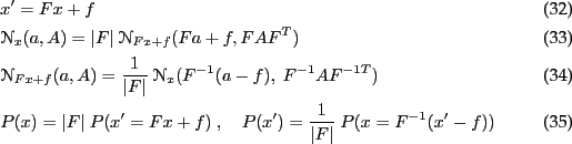
Let there be ![]() random variables
random variables ![]() . We assume that the joint
probability can be written as a product of
. We assume that the joint
probability can be written as a product of ![]() factors
factors
![]() where
where ![]() is a tuple of indices in
is a tuple of indices in ![]() specifies the variables the
specifies the variables the ![]() th factor depends on
th factor depends on
![]()
In the infer package, different types of factores are provided: tables, Gaussians, MoGs, Gaussians with quasi-non-linear dependencies, etc - see below. But the basic operations on the factor graph discussed in this section are largely independent of the type of factors.
Actually, providing the list of factors ![]() and the list of tuples
and the list of tuples
![]() is sufficient to fully determine a model. Based on this, some
algorithms could analyze the dependencies, e.g., find a Junction Tree,
and thereby decide on elimination orders etc. The result of such
analysis would be arcs between factors. We include this in the basic
data structure.
is sufficient to fully determine a model. Based on this, some
algorithms could analyze the dependencies, e.g., find a Junction Tree,
and thereby decide on elimination orders etc. The result of such
analysis would be arcs between factors. We include this in the basic
data structure.
Let ![]() be a graph with
be a graph with ![]() nodes. The
nodes. The ![]() th node is associated with
the factor
th node is associated with
the factor ![]() . Additionally the graph contains edges
. Additionally the graph contains edges ![]() between
nodes.
between
nodes.
For each edge ![]() we can compute the intersection of random
variables that
we can compute the intersection of random
variables that ![]() and
and ![]() depend on; we use
depend on; we use ![]() to denote
the index tupel of this intersection,
to denote
the index tupel of this intersection,
![]()
The random variables
![]() are the basis of
communication between the factors
are the basis of
communication between the factors ![]() and
and ![]() in belief
propagation type algorithms - the factors will exchange their beliefs
on the marginal of
in belief
propagation type algorithms - the factors will exchange their beliefs
on the marginal of
![]() .
.
As the final part of the basic data structure, we also associate two
factors to each adge - one as a memory for forward messages and one
for backward messages. We denote them by
![]() and
and
![]() .
.
The data structure consists of a graph withnodes and some edges. For each node we have
and for each edge we have
.
As abbreviation we write
![]()
States of the data structure
Let's define the data structure is...
- junction complete
- if there always is an edge
 , when
 and
and  share variables
- a junction tree
- if a junction complete tree and all junctions
 are disjoint (`running intersection property')
- bipartite
- if the factors can be separated in single variable
factors and clique factors and only interconnections (no
intra-connections) between the groups are present
- in initial state
- if all
 such that one can
(redundantly) write
such that one can
(redundantly) write
- consistent
- with the original factors
 if the
current factors and incoming messages
if the
current factors and incoming messages  fulfill
Note that in this case
and the original joint is still correctly encoded in the data structure. - in equilibrium
- if all factors and edges agree on the junction
marginals, which is
The infer package includes routines to check the state of the data structure, i.e., whether it is still consistent or in equilibrium. These are an important tool for debugging.
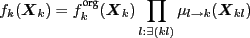
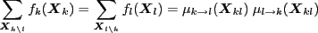
Message exchange
Say ![]() and
and ![]() share some variables and let
share some variables and let ![]() and
and ![]() be their marginals w.r.t. these shared variables. A (directed!)
message exchange from a factor
be their marginals w.r.t. these shared variables. A (directed!)
message exchange from a factor ![]() to another
to another ![]() is (dashes mean
reassignments):
is (dashes mean
reassignments):
The updates are written in many different forms to see alternatives
for the implementation. Intuitively: The message ![]() reflects the
marginal of
reflects the
marginal of ![]() leaving out all information that has previously been
exchanged between
leaving out all information that has previously been
exchanged between ![]() and
and ![]() .
. ![]() `summarizes' all
messages that have yet been send from
`summarizes' all
messages that have yet been send from ![]() to
to ![]() . Alternative
thinking: The quotients
. Alternative
thinking: The quotients
![]() and
and
![]() that appear in these equations are the original (initial state)
factors multiplies with all incoming messages
except for the ones from
that appear in these equations are the original (initial state)
factors multiplies with all incoming messages
except for the ones from ![]() and
and ![]() , respectively,
, respectively,
![]()
Note that this message exchange preserves consistency because
![]()
Second, note that in equilibrium
![]() and thus
and thus ![]() and the message exchange has no effect.
and the message exchange has no effect.
Approximate message exchange
[[ realized yet for MoGs ]]
On factor graphs with mixture of Gaussians (say a Markov chain/switching state space model), the marginal of a factor usually contains more Gaussian modes than a message can represent (the number of models would grow exponentially on a Markov chain). Hence, marginalization for a MoG is implemented approximate by collapsing all Gaussians that correspond to the same mixture component.
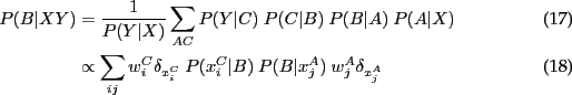
Approximate message exchange (e.g., expectation propagation / assume density filtering)
Factors or messages are sometimes limited to represent only a class of
distributions (e.g., Gaussians in the continuous case), then one might
not be able to do an exact message exchange because ![]() is not
in this class of distributions. The approximate message exchange then
is
is not
in this class of distributions. The approximate message exchange then
is
![]()
where the approximation refers to some Assumed Density
Filtering approach. In this case, the message factors ![]() should be updated according to
should be updated according to
![]()
because only this update preserves consistency (
![]() would not because of the approximation).
would not because of the approximation).
Mean field approximations
[[ todo ]]
Given a graph with only two factors ![]() and
and ![]() . A mean field
approximation would compute the current b
. A mean field
approximation would compute the current b
Mean field approximations take the
Particle filtering
[[ Nando's paper: Fast Particle Smoothing: If I had a million particles
How can you rearrange particles from the forward and backward filter? ]]
Think of the Markov chain
![]() with arbitrary
continuous transitions and observations
with arbitrary
continuous transitions and observations ![]() and
and ![]() .
. ![]() is
represented as a population (fwd particle filter),
is
represented as a population (fwd particle filter), ![]() is
represented as a population (backwrad particle filter). I want
is
represented as a population (backwrad particle filter). I want
Factors
Generic operations and testing
To implement inference algorithms, only a few basic operations need to
be provided to manipulate factors (![]() 's and
's and ![]() 's). These are
's). These are
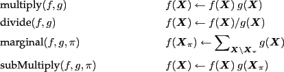
and for practical reasons also some more trivial methods
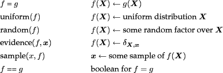
In the implementation, a class factor will define these methods as virtuals. Factor implementations derived from this base class implement these methods.
A robust way to check the validity of a factor implementation is to define tests in the spirit of unit testing. We define that a valid factor has to pass the following randomized tests:
Let ![]() and
and ![]() be two cliques of variables, each with a
random number
be two cliques of variables, each with a
random number ![]() of variables, each variable with random
dimensionality/cardinality, and with sharing random variables
of variables, each variable with random
dimensionality/cardinality, and with sharing random variables ![]() .
.
![\begin{test}[multiply, devide]
\item $f(X_k)$\ = random,~ $h(X_k)$\ = random
\item assert~ $f*h=h*f$\ ~ and ~ $(f * h)/h = f$\ ~ and ~ $(f*h)/f = h$
\end{test}](img92.png)
![\begin{test}[message passing]
\item $f(X_k)$\ = random,~ $h(X_l)$\ = random
\ite...
...wd between $f$\ and $h$
\item assert $f$\ and $h$\ are in equilibrium
\end{test}](img93.png)
![\begin{test}[marginal]
\item $f(X_k)$\ = random,~ $h(X_{kl})$\ = random
\item $g...
...pi_{kl})$
\item $g'$\ = marginal$(f',\pi_{kl})$
\item assert $h*g=g'$
\end{test}](img94.png)
Some factor implementations will pass these tests only approximately. E.g., a mixture of Gaussians can pass test 1 and 2, but not exactly test 3.
Factor types
Tables
![]() is discrete and
is discrete and ![]() is stored as a table. The
operations are conceptually straightforward to implement.
is stored as a table. The
operations are conceptually straightforward to implement.
In practice, to store a table factor one should always store a table
![]() scaled to sum to 1 and additionaly a log scaling
scaled to sum to 1 and additionaly a log scaling ![]() such
that
such
that
![]()
In that way, over- and underflow in the table is buffed in the scaling
![]() . (In HMMs, e.g.,
. (In HMMs, e.g., ![]() will end up being the data log-likelihood.)
will end up being the data log-likelihood.)
Gaussians
![]() is a continuous variable and
is a continuous variable and
![]() .
Product, devision and marginal product are best implemented in the
canonical representation
.
Product, devision and marginal product are best implemented in the
canonical representation
![]() . Only the marginal
extraction requires matrix inversions, which are the Schur
complements: The marginal precision matrix for
. Only the marginal
extraction requires matrix inversions, which are the Schur
complements: The marginal precision matrix for ![]() for a joint
precision matrix
for a joint
precision matrix ![]() is
is
![]() . See the
appendix for details.
. See the
appendix for details.
Again, in addition to the ![]() and
and ![]() we store a scaling
we store a scaling
![]() such that
such that
![]()
Mixture of Gaussians
[[implemented]]
Unscented Transform Gaussian factor
Two variables ![]() and
and ![]() , Gaussian over
, Gaussian over ![]() , a generic (non-linear)
but invertible(!) function from
, a generic (non-linear)
but invertible(!) function from ![]() to
to ![]() . Using the UT to map from
. Using the UT to map from
![]() to
to ![]() and back.
and back.
[[implemented]]
Linearized Function Gaussian factor
Two variables ![]() and
and ![]() , Gaussian over
, Gaussian over ![]() , a generic (non-linear,
perhaps redundant) function from
, a generic (non-linear,
perhaps redundant) function from ![]() to
to ![]() which provides a local
linearization (the Jacobian). The fwd mapping from
which provides a local
linearization (the Jacobian). The fwd mapping from ![]() to
to ![]() is
trivial using the linearization around the mean of
is
trivial using the linearization around the mean of ![]() . The backward
mapping is tricky in the case of redundancy:
. The backward
mapping is tricky in the case of redundancy:
- Linearize around the mean of
 (the must be some meaningful
prior on otherwise it doesn't work!),
(the must be some meaningful
prior on otherwise it doesn't work!),
- redundantly pull back the Gaussian on
 , blowing up variance
along the null space,
, blowing up variance
along the null space,
- execute multiplication with ,
- relinearize the function and the new mean, and repeat from (ii)
[[implemented]]
Switch factors for relational/logic models
Consider ![]() random variables
random variables ![]() of same type (in the same
space) and a discrete random variable
of same type (in the same
space) and a discrete random variable
![]() . Given
. Given
![]() and
and ![]() , we have another random variable
, we have another random variable ![]() which depends
only on
which depends
only on ![]() :
:
![]()
In general terms, ![]() depends on all
depends on all ![]() and
and ![]() and we have
and we have
![]() . The definition above though captures much
more structure in this dependency.
. The definition above though captures much
more structure in this dependency.
We introduce switch factors
![]() to `copy' the random
variables
to `copy' the random
variables ![]() into an additional buffer random variable
into an additional buffer random variable ![]() . That
way we can then introduce a simple factor for
. That
way we can then introduce a simple factor for ![]() .
.
A switch factor is of the form
![]()
where ![]() and
and ![]() store marginal factors over
store marginal factors over ![]() and
and ![]() respectively.
respectively.
It should be possible to implement all core methods.
[[work in progress]]
Decision tree factor
[[not approached yet]]
Particle factors
[[ideas, but not approached yet]]
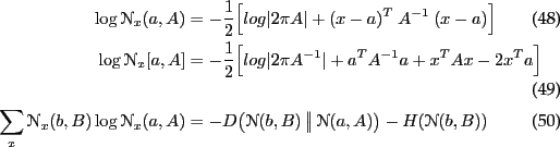
Appendix: Gaussians
Definitions
In normal form
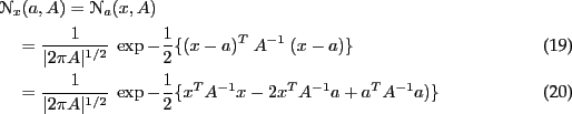
In canonical form (with
![\begin{align}
&\NN_x[b,B]
= \NN_x(B^{-1} b,B^{-1})
= \frac{\exp-\half\{b^T B^{...
...}{\vert 2\pi B^{-1}\vert^{1/2}}~ \exp
-\half\{x^T~ B~ x - 2 x^T b\}
\end{align}](img117.png)
Non-normalized (e.g., for propagating likelihoods)
Matrices
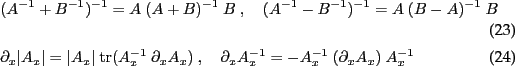
Derivatives
Product
![\begin{align}
\NN_x&(a,A) \cdot \NN_x(b,B) = \NN_x(c,C) \cdot \NN_a(b,A+B) \feed...
...\quad= \NN_x[a+b,A+B] \cdot \NN_{A^{-1}a}[A(A+B)^{-1}b,A(A+B)^{-1}B]
\end{align}](img121.png)
Division
![\begin{align}
\NN_x&(a,A) ~\big/~ \NN_x(b,B) = \NN_x(c,C) ~\big/~ \NN_c(b,C+B) \...
...} - B^{-1} \\
\NN_x&[a,A] ~\big/~ \NN_x[b,B] \propto \NN_x[a-b,A-B]
\end{align}](img122.png)
Transformation
block-matrices
![\begin{align}
&\left\vert\arr{cc}{A&C\\ D&B}\right\vert = \vert A\vert~ \vert\ba...
...1}&-\bar A^{-1} C B^{-1}\\ -B^{-1} D \bar A^{-1}&\bar B^{-1}}\right]
\end{align}](img124.png)
marginal & conditional:
We write
![\begin{align}
\left[\arr{c}{x\\ y}\right] \sim \{ \left[\arr{c}{a\\ b}\right] , ...
... Fa+f}\right] ,~ \left[\arr{cc}{A&A^T F^T\\ FA&Q+F A^T F^T}\right]\}
\end{align}](img131.png)
![\begin{align}
\left[\arr{c}{x\\ y}\right] \sim [ \left[\arr{c}{a\\ b}\right] , \...
...\\ h}\right] ,~
\left[\arr{cc}{A+H^T B^{-1} H&-H^T\\ - H&B}\right]]
\end{align}](img132.png)
Entropy
Kullback-Leibler divergence
![]() -divergence
-divergence
![]()
For ![]() : Jensen-Shannon divergence.
: Jensen-Shannon divergence.
Log-likelihoods
Mixture of Gaussians
Collapsing a MoG into a single Gaussian

Marginal
![\begin{align}
&P(x,y) = \sum_i p_i~ \NN_{x,y}(\left[\arr{c}{a_i\\ b_i}\right],\l...
...i~ B_i^{-1} C_i^T \comma
f = \sum_i p_i~ B_i^{-1} b_i \comma
Q = ?
\end{align}](img140.png)
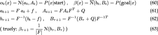
Kalman filter (fwd) equations
linear fwd-bwd equations without observations
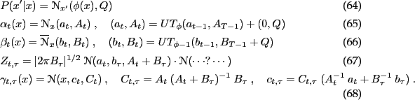
non-linear fwd-bwd equations without observations
About this document ...
Inference and planning on factor graphs- technical notes -
- draft -
This document was generated using the LaTeX2HTML translator Version 2002-2-1 (1.71)
Copyright © 1993, 1994, 1995, 1996,
Nikos Drakos,
Computer Based Learning Unit, University of Leeds.
Copyright © 1997, 1998, 1999,
Ross Moore,
Mathematics Department, Macquarie University, Sydney.
The command line arguments were:
latex2html -split 0 -no_navigation index.tex
The translation was initiated by mt on 2007-07-18
mt 2007-07-18