supplements for IJCAI 05
This page contains some supplementary materials to a paper submitted
to IJCAI 05: Marc Toussaint & Sethu Vijayakumar:
Learning discontinuities for switching
between local models. These are mainly larger graphs and more
experimental results than the limited length of the paper
permitted. Please refer to this paper for more details.
1D test function - data and learned switching model
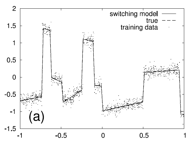
The following graph displays noisy data from a 1D test function. The
dashed line is the underlying test function without noist. E.g., in
the interval [-.5,-.2] one can see a significant deviation between the
true test function and the function learned by our model. Clearly, the
reason is that the noise hardly allows to infer that the true test
function has an extra step. In total, the test function is composed of
10 pieces and 1000 data points were used.
1D test function - blended switching model and LWPR
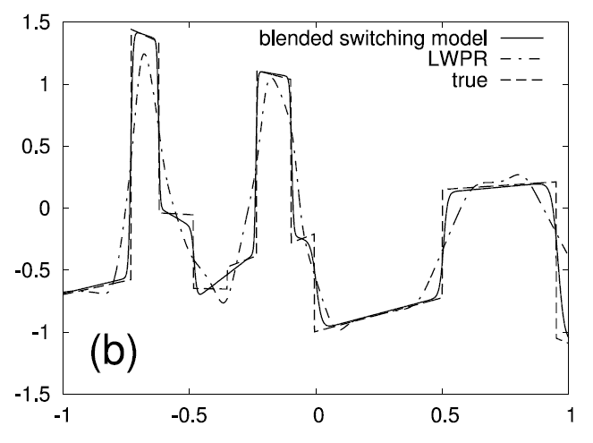
The next graph displayes the same 1D test function (dashed line) and a
learned switching model (cont. line). But here, the output of the
learned model is given as the weighted average of the outputs of the
family members ‐, weighted by the coefficient beta. Strictly
speaking, this is not conform with the probabilistic framework, which
says that beta is a probability associated with a model, and not an
averaging coefficient. Still, the graph allows to see the sigmoids
that are actually behind the switching.
The dash-dotted curve
displays the function learned with LWPR, which allocated 15 kernels to
represent this function. Clearly, LWPR is not designed to learn
discontinuities.
Family and classification errors for 2D, 5D, and 10D test
functions
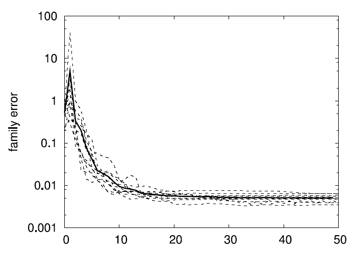
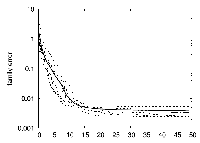
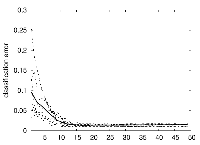
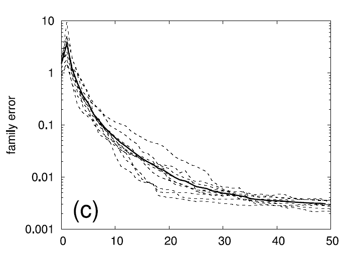
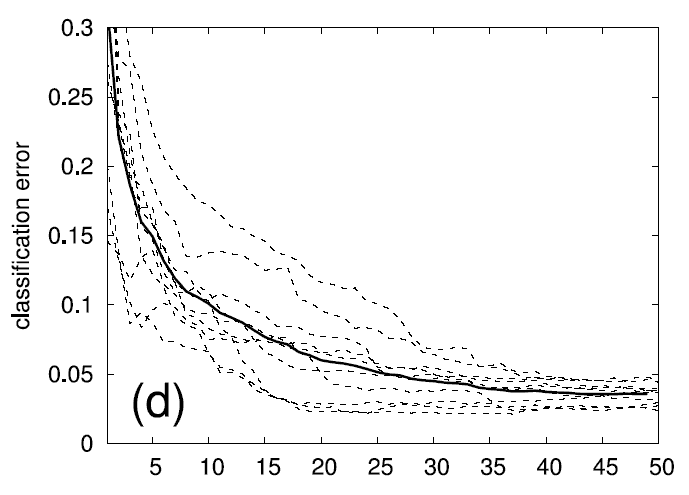
The following graphs display what we call the
family error and
the
classification error. The family error only evaluates the
quality of the family of models independent of how well the second
level of the algorithm (the product of sigmoids) can predict which
model gives the best output. For every data point, it simply evalues
the MSE of the best fitting eligible model within the family. This is
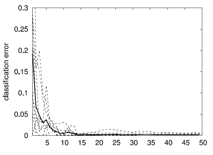
averaged over a whole test data set. In contrast, the classification
error indicates the quality of the second level of the algorithm by
counting how often the product of sigmoids do indeed predict the
correct model as being the best for a given (input) datum. The error
is given as a percentage over the a test data set. E.g., a family
error of .01 and a classification error of 4% means that in 96% of
the test data points, the model chose correctly the best fitting model
from the family, which has, on average, an MSE of .01 (which is
optimal given the noise level).
The following two graphs display 10 runs over random 2D test
functions with training data set size 1000. The bold lines are the
averages over the 10 independent runs.
The following two graphs display 10 runs over random 5D test
functions with training data set size 10000. The bold lines are the
averages over the 10 independent runs.
The following two graphs display 10 runs over random 10D test
functions with training data set size 10000. The bold lines are the
averages over the 10 independent runs.
Recent Posts
Die gängigen Erklärungen zu “Was ist Informatik?” – etwa von der
Gesellschaft für Infomatik,
der
TU Dresden,
oder auf Wikipedia –
machen es einem schwer, sic...