Monte Carlo methods are the techniques which used in computing estimates via sampling. These methods are highly used within the range from estimating of a intractable integral to system simulation. Here, I’ll try to give some initial ideas with the help of the illustration of some basic techniques.

We can start with inversion method. The key idea of it is that when $f_X$ is the probability density of the random variable $X$, the cumulative density function (CDF) $F_X(X)$ is uniformly distributed on [0, 1) when viewed as a random variable. Thus, if we choose uniform $U$ and obtain $X$ by $X = F_X^{-1}(U)$, the density of $X$ will be $f_X$. To examplify, we try to get uniform samples from a circle. For this, we have 2 random variables, for radial and angular coordinates; and CDF function:

$R \sim p({r}) = 2r$ for $0 \leq r \leq 1$

$\Theta \sim U(\theta; 0, 2\pi)$.

$F_R({R}) \sim \int_0^r2xdx=r^2$ and $F_R^{-1}(U) \sim \sqrt u$

Thus, taking a value on uniform probability density on [0, 1] and square root of it gives sample from $p({r})$.

import random
import numpy as np
import matplotlib.pyplot as plt

N = 5000
r = [np.sqrt(random.random()) for i in range(N)]
theta = [random.random() * 2 * np.pi for i in range(N)]

x = np.multiply(r,np.cos(theta)) 
y = np.multiply(r,np.sin(theta)) 

plt.plot(x, y, ’k.’,label = ’’)
plt.xlabel(’x’)
plt.ylabel(’y’)
plt.legend()
plt.show()

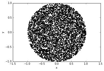
At the end, we are able to get uniform samples from a 2-norm unit ball ($x^2 + y^2 = 1$).

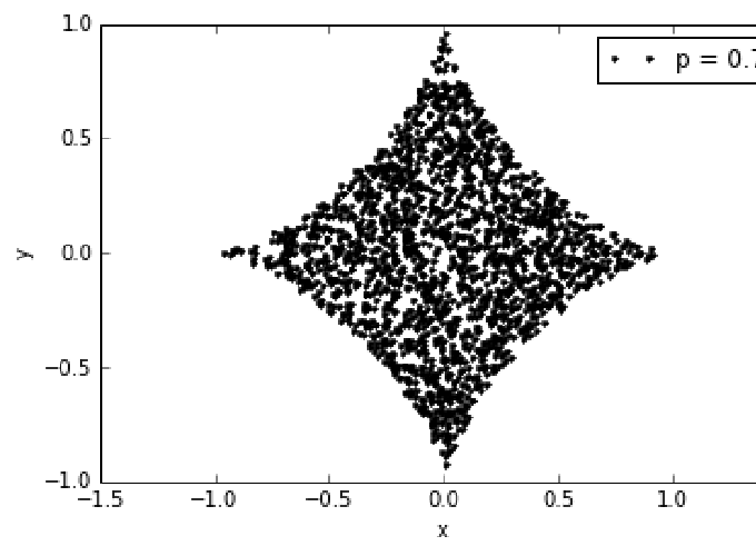
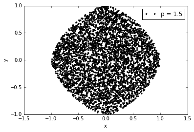
But, if we want to get uniform samples from an another p-norm unit ball ($(|x|^p + |y|^p)^{1/p} \leq 1$), we can use rejection sampling. It is an another method for indirectly sampling from a target distribution by sampling from a proposal distribution. We reject some of the generated samples to compensate for the fact that target and proposal distributions are not equal with some acceptance/rejection probability. For instance, we can draw samples from the closed unit ball for $p = 1.5$ like that:

x_list = []
y_list = []
count = 0.0
for j in range(N):
    r = np.sqrt(random.random())
    theta = random.random() * 2 * np.pi
    x = np.multiply(r, np.cos(theta))
    y = np.multiply(r, np.sin(theta))
    check = np.power(np.power(np.absolute(x),1.5) + np.power(np.absolute(y), 1.5), np.divide(1, 1.5))
    if check <= 1:
        count += 1.0
        x_list.append(np.multiply(r, np.cos(theta)))
        y_list.append(np.multiply(r, np.sin(theta)))
plt.axis(’equal’)
plt.plot(x_list, y_list, ’k.’,label = ’p = ’+str(i))
plt.xlabel(’x’)
plt.ylabel(’y’)
plt.legend()
plt.show()
print 'Acceptance Rate =', np.divide(count,N)

Acceptance rate = 0.8668

These are just very toy examples but I hope this post gives some initial ideas about Monte Carlo methods. For those who want to continue with this subject, I suggest [A Tutorial Introduction to Monte Carlo Methods, Markov Chain Monte Carlo and Particle Filtering](https://www.researchgate.net/publication/288191971_A_Tutorial_I